Trigonometric Graphs | Functions, Units Of Angle, Examples

Contents hide

3 Trigonometric function and the unit circle

Introduction

What do you get when you join three distinct points, that are not located on a single line, in a plane? That is right, a triangle. Triangles appear to be simple and innocent. In fact, a triangle is the simplest polygon (a closed 2-D shape with straight sides). Ironically, in mathematics there is a dedicated branch for the study of relationships between sides and angles of these simple three-sided shapes. Trigonometry (from trigonon, “triangle” and metron, “measure”) is the name of that branch.

Right Triangle

You may recall that the sum of the three angles of a triangle is equal to $180^{\circ}$ . If one of the angles of the triangle is equal to $90^{\circ}$ , the triangle is called the ‘right triangle’. Right triangles have some unique properties. You may remember the famous Pythagoras theorem i.e., for a right triangle, the sum of the squares of the length of the sides opposite to the smaller angles is equal to the square of the length of the side opposite to the right angle i.e.,

$a^{2}=b^{2}+c^{2}$

Figure 1 A right triangle with side lengths a, b and c

Interesting fact: You can split any triangle into two right triangles by dropping a perpendicular on a side from a corner/vertex of that triangle.

Trigonometric functions

Other than the right angle, the inner angles of a right triangle are related to the length of its sides. Consider the right triangle in figure above. We observe that the angle between the sides a and c is related to the length of the sides. Variation of the length of the sides results in variation of the angle .

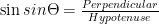
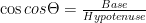
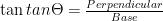
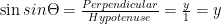
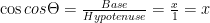
Trigonometric functions are used to express those relations. The three basic trigonometric functions have been defined as the ratio of the sides of a right triangle. The ratio is dependent on the angle θ, therefore, the basic trigonometric functions are represented as the functions of angle θ. They are:

$\sin sin\Theta = \frac{Perpendicular}{Hypotenuse}$

$\cos cos \Theta = \frac{Base}{Hypotenuse}$

$\tan tan \Theta = \frac{Perpendicular}{Base}$

Question: Can you find a relationship between these three trigonometric functions?

Here are some key points to note. We can see that for a right triangle,

Hypotenuse ≥ Perpendicular

Hypotenuse ≥ Base

This means that the sin sin θ (pronounced as sine of theta) being the ratio of perpendicular and hypotenuse can have a maximum value of 1. Same goes for cos cos θ (or cosine θ) . As far as tan tan θ (or tangent θ) is concerned, we can see that it is the ratio of perpendicular and base which can vary between 0 (when perpendicular = 0) and infinity (when base = 0).

There are three other trigonometric functions defined as:

$cosec\Theta = \frac{1}{\sin sin \Theta }=\frac{Hypotenuse}{Perpendicular}$

$\sec sec\Theta = \frac{1}{\cos cos \Theta }=\frac{Hypotenuse}{Base}$

$\cot cot\Theta = \frac{1}{\tan tan \Theta }=\frac{Base}{Perpendicular}$

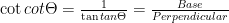
Note that cosecant, secant and cotangent are the full forms of cosec, sec and cot respectively.

Units of angle

The angle is either presented in the units of degrees or radians. Remember that,

2π radians = 360 degrees

But what is this radian and why the relation holds? The concept of radian is interesting.

As it can be noted that there is no liaison between degrees and the unit of length (they are totally different). The idea of radian is introduced to fill that gap. Consider a pivoted line of length ‘r’ that traces an arc through an angle ‘θ’. The length ‘l’ of the arc is related to the angle and r by the following relation:

l = rθ

We see that l = r when θ = 1. This is the definition of a radian! i.e., the angle through which a line of length ‘r’ should move to trace an arc of equal length. In exactly 2π radians, whole circle can be traced out. Now you know why the circumference of a circle is 2πr.

Question: How many degrees are there in one radian?

Trigonometric function and the unit circle

Now that we have established relationships between the angle θ and side lengths of a right triangle in the form of trigonometric functions, and also understood the concept of radian, we can extend the discussion.

Imagine a unit circle (circle with radius of 1) in xy plane centered at the origin. The line connects a point with coordinates (x, y) on the circle to the origin (0,0). The line forms an angle θ with the x-axis. From the figure we can see that a right triangle can be constructed. Since the coordinates of the point are (x,y), the side lengths of the right triangle are x and y. Using the Pythagoras theorem, we can see that $x^{2}+y^{2}=1$ , which is in fact the equation for the circle.

Figure 2 Right triangle in a unit circle

Using the definition of sine and cosine, we have:

$\sin sin\Theta = \frac{Perpendicular}{Hypotenuse}=\frac{y}{1}=y$

$\cos cos \Theta = \frac{Base}{Hypotenuse}=\frac{x}{1}=x$

i.e., $\sin sin\Theta = y$ and $\cos cos \Theta = x$ . You should have realized that by using the original definition of trigonometric functions, we cannot find the value of the function for $\Theta > 90^{\circ}$ or $\frac{\pi }{2}$ . The expressions $\sin sin\Theta = y$ and $\cos cos \Theta = x$ (where x and y are coordinates of the circle) can be used to find the value of trigonometric function for $\Theta > 90^{\circ}$ or $\frac{\pi }{2}$ .

We observe that as the line traces the circle, the angle varies form 0 to 360 degrees (or 2π radians). It is important to introduce the idea of ‘Quadrant’ here.

A quadrant is one fourth of the infinite xy cartesian plane when divided based on the sign (positive/negative) of x and y axes. Thus, we have a total of four quadrants:

First quadrant (Quadrant-I) – Positive x and Positive y ( $0^{\circ}\leq \Theta \leq 90^{\circ}$ )
Second quadrant (Quadrant-II) – Negative x and Positive y ( $90^{\circ}\leq \Theta \leq 180^{\circ}$ )
Third quadrant (Quadrant-III) – Negative x and Negative y ( $180^{\circ}\leq \Theta \leq 270^{\circ}$ )
Fourth quadrant (Quadrant-IV) – Positive x and Negative y ( $270^{\circ}\leq \Theta \leq 360^{\circ}$ )

Quadrants have been labelled in Figure 2. Using the expressions; $x = \cos cos \Theta$ and $y= \sin sin\Theta$ , we can find the sign of the trigonometric functions in different quadrants.

In the first quadrant $0^{\circ}\leq \Theta \leq 90^{\circ}$ , both x and y coordinates are positive. Therefore, both cosine and sine of θ are positive. Also, the $\tan tan \Theta$ is positive because $\tan tan \Theta = \frac{Perpendicular}{Base}=\frac{y}{x}$ .
In the second quadrant $90^{\circ}\leq \Theta \leq 180^{\circ}$ , x is negative and y is positive. Therefore, $\cos cos \Theta$ is negative, $\sin sin\Theta$ is positive and $\tan tan \Theta$ is negative.
In the third quadrant $180^{\circ}\leq \Theta \leq 270^{\circ}$ , both x and y are negative. Therefore, both $\cos cos \Theta$ and $\sin sin\Theta$ are negative, whereas $\tan tan \Theta$ is positive.
In the fourth quadrant $270^{\circ}\leq \Theta \leq 360^{\circ}$ , x is positive while y is negative. Therefore, $\cos cos \Theta$ is positive, $\sin sin\Theta$ is negative and $\tan tan \Theta$ is also negative.

To remember this, you can develop a mnemonic with letters “ASTC” (All positive in Quadrant-I, only Sine positive in Quadrant -II, only Tangent positive in Quadrant-III, only Cosine positive in Quadrant-IV).

The reader should observe that the sine and cosine vary between -1 and 1, whereas tangent varies between -∞ and ∞ (since $\tan tan \Theta =\sin sin\Theta \setminus \cos cos \Theta$ ), when θ varies from 0 to 2π radians (or $360^{\circ}$ ). What happens when θ is increased beyond 2π? Well, imagine the unit circle.

The line rotating around its center starting from 0 in 1st quadrant. It moves into the 2nd quadrant after crossing π/2 radian line, then it moves into the 3rd quadrant after crossing , then 4th quadrant after crossing $\frac{3\pi }{2}$ radian line and finally reaches the starting point i.e., point (1,0) by overlapping on the x axis. It is evident that further increasing the angle would result in ‘repetition’ of the whole ‘cycle’. This property of trigonometric functions called ‘Periodicity’ makes them extremely significant.

We say that 2π is the period of $\sin sin\Theta$ and $\cos cos \Theta$ (and of cosec θ and sec sec θ), whereas that of $\tan tan \Theta$ (and $\cot cot \Theta$ ) is π (we will explore this later in this article). After 2π (for sine and cosine) and π (for tangent), the values of trigonometric functions start repeating. Note that 2π is not always the period of the trigonometric functions $\sin sin\Theta$ and $\cos cos \Theta$ . For instance, the period of $\sin sin2\Theta$ is π or $180^{\circ}$ . It is because when θ = π, 2θ = 2π. You can see that the 2 in 2θ is responsible for the period being equal to π.

Questions: Find the period of:

$\sin sin \frac{2\Theta}{3}$
$\cos cos 0.5\Theta$
$\tan tan \frac{\Theta}{4}$

The concept of periodicity will help in graphing of trigonometric functions.

Graph of Trigonometric Functions

Now that we have developed a sound foundation in trigonometry, let us graph the trigonometric functions. Believe that graphs of sine, cosine and tangent are a piece of cake. By the end of this article, you will not be afraid of sketching plot of any trigonometric function. Familiarity with the following ideas will help us.

Amplitude of a function
Period of a function
Phase angle
Mean or Center value of a function

After that we have gone through the concept of periodicity and the fact that $\sin sin\Theta$ and $\cos cos \Theta$ vary between -1 and 1, the reader can imagine that the graphs of $\sin sin\Theta$ and $\cos cos \Theta$ would include oscillations, right? Also, there would also be a center of oscillation (called the mean).

We have a rough outline in our minds now. Let us grab a calculator and knowing the fact that the period is 2π, we evaluate the function $\sin sin\Theta$ at 6-7 different values of angle between 0 and 2π.

Caution: A very common mistake that students make, is with the settings of unit of angle in their calculators. Always check the settings before evaluating the trigonometric functions. Whatever the unit is set, input the value accordingly e.g. If the unit is set to radian then the calculator would consider the input as radians i.e., if you input 180, it would evaluate sine of 180 radians (not degrees).

Here are some values of the function $\sin sin\Theta$ at different angles,

0	0
π/4	0.7071
π/2	1
3π/4	0.7071
π	0
5π/4	-0.7071
3π/2	-1
7π/4	-0.7071
2π	0

These points can be marked on a graph paper and then joined by hand smoothly. The curve can be extended beyond 2π by repeating the pattern (since 2π is the period of $\sin sin\Theta$ ). Ultimately, we get a graph that looks like this,

Note that beyond 2π, the plot repeats indefinitely. The mean or center of the plot is 0 (since the graph oscillates around 0). The amplitude is 1 (maximum distance between center and extreme value of the function).

Let us now play around with it. What would the graph of $2\sin sin\Theta$ look like? To answer this, try to see how is this function different from $\sin sin\Theta$ . We note that,

It is only scaled by a factor of 2.
The period has not changed (no constant multiplied with θ).
The mean/center is still 0 (no shifting along y-axis i.e., no number added in the function)
The phase angle is still 0 (no shifting along x-axis i.e., no number added in the input of the function)

We can immediately draw the graph for $2\sin sin\Theta$ by hand. It looks like

See, that was easy and intuitive!

Now graph the function $\sin sin2\Theta$ . Wait, have we not graphed it already? No, look closely.

You might have guessed now that the period has halved. Therefore, the graph should have squeezed by a factor of 2. Imagine it now, the squeezed sine wave! Good. Now draw the graph by hand on the graph paper. It should look like

Piece of cake, right? See how the function $\sin sin2\Theta$ completes a cycle in only π radians.

Let us move ahead. What is the mean/center of the functions we have been plotting? That is 0 (Take your time to get yourself comfortable with this idea). Now if it is asked to ‘shift’ the curve of $\sin sin\Theta$ by one unit up i.e., translate every point on the graph of $\sin sin\Theta$ one unit up, it will be the same as asking to plot the function $\sin sin\Theta+1$ . The plot will look like

To plot it accurately by hands, there is a little trick. Plot the usual sin θ by hand with the center x-axis dotted. Label the axis by the magnitude it has been translated up or down (‘1’ in this case). Considering the amplitude of the function (1 in this case), locate the original x-axis and draw it with a solid line. You should realize that the amplitude of θ)+1 ” is still 1 (not 2, the maximum value on the graph). It is because as discussed earlier, the amplitude is maximum distance between mean/center and the extreme values. The mean/center of θ) +1 is also 1 because it can be seen that the graph of θ)+1 oscillates around 1.

How do we translate the graph along the x-axis? That is right. Add something in the input of the function. This is basically the idea of phase angle. You can consider phase angle as an offset angle for the trigonometric function. For instance, the function $\sin sin\Theta$ evaluates at the same values of θ (that we input) without any offset (its phase angle is 0).

On the other hand, consider the function $\sin sin(\Theta-\frac{\pi }{4})$ . When we input θ = 0 radians, the function is evaluated as $\sin sin(\Theta-\frac{\pi }{4}))=\sin sin(-\frac{\pi}{4})$ .

At $\Theta = \frac{\pi}{4}$ , the function $\sin sin(\Theta-\frac{\pi }{4}) = \sin sin(\frac{\pi }{4}-\frac{\pi }{4})=0$ .

At $\Theta = \frac{\pi}{2}$ , the function $\sin sin(\Theta-\frac{\pi }{4}) = \sin sin(\frac{\pi }{2}-\frac{\pi }{4})=sin sin(\frac{\pi }{4})$ . Thus, the graph translates along the x-axis.

Question: The graph of $\sin sin\Theta$ translates towards left or towards right for $\sin sin(\Theta-\frac{\pi }{4})$ ? Guess before looking at the next plot!

Did it translate towards positive x-axis? The answer is “yes”. You may recall that the graph translated along positive y-axis when we had added a positive number in the original function. But in this case, the graph translated along positive x-axis when we added a negative number in the angle. Also, note the difference between two types of translation:

(sin sin θ) + a (Translation along the y-axis)
sin sin (θ+a) (Translation along the x-axis)

where a can be positive or negative real number.

Till now, we have covered four cases:

Scaling with respect to y-axis,
Scaling with respect to x-axis,
Translation along y-axis,
Translation along x-axis.

You may have realized that you even do not have to use the calculator now, for the plot of sine function.

Questions: Put your understanding to test by sketching the graphs of following functions:

θ
$\sin sin(0.2\Theta)$
$0.2 + \sin sin \Theta$
$\sin sin (\Theta + 0.2)$

You can also plot functions involving combinations of scaling and translation along the two axes. This is intuitive to do. You just have to ‘superimpose’ the concepts you have learnt. For instance, to plot a + sin⁡(bθ), you can sketch the plot of sin⁡(bθ) as the first step, then translate it by ‘a’ units along the y-axis. Try the following functions:

$1.5 + 0.5\sin sin\Theta$
$2\sin sin(0.5\Theta)$
$3sin(2\Theta-1)$

Graph of cosine function

You have already got this. The graph of sine and cosine are the same except the fact that they are shifted along the x-axis with respect to each other. The graph of cosine is presented below:

Figure 8 Graph of cos cos θ and sin sin θ

In order to not mix up the two plots, note that cos⁡0 is 1 (You can imagine the unit circle, and the line with an angle of 0. The line is connected to the point (1,0) i.e., x=1. Also, recall that x = cosθ. Thus, cos 0 = 1). In short, the graph for sine starts from 0 at θ = 0 and that of cosine starts from 1.

Question: The graph of cosine looks like shifted sine graph, by an angle of π/2. Can you develop a relation between sine and cosine based on the concept of phase angle, just by looking at the graph?

All the four transformations i.e., translation and scaling apply to other trigonometric functions equally well. We do not need to discuss that again. However, as practice try to plot the following functions:

$cos (2\Theta)$
$1+2cos \Theta$
$0.5+3cos (\Theta +1)$

Graph of tangent

The function $\tan tan \Theta$ is quite different, as it is the ratio of $\sin sin\Theta$ and $\cos cos \Theta$ . Let us take a look at the graph of $\tan tan \Theta$ and discuss its features.

Indeed, as you can see it is nothing like what we have previously seen. To explain the details of this graph, let us redraw it with overlapped graphs of $\sin sin\Theta$ and $\cos cos \Theta$ .

Figure 10 Graph of tan θ, sin θ and cosθ

Starting from θ=0, sine is 0 and cosine is 1. Therefore, $\tan tan \Theta$ being the ratio of sine and cosine is 0/1 = 0. From 0 to π/2, the value of $\sin sin\Theta$ increases from 0 to 1 while that of $\cos cos \Theta$ decreases form 1 to 0. As a result, $\tan tan \Theta$ increases monotonically from 0 to ∞.

Note that $\tan tan \Theta$ is undefined for θ = π/2.

As becomes greater than π/2 or $90^{\circ}$ , cosine becomes negative (recall the “ASTC” mnemonic), while sine stays positive. The magnitude of sine varies (from 1 to 0), whereas that of cosine varies from (0 to -1). Therefore, the $\tan tan \Theta$ flips its direction as just crosses π/2 mark and monotonically varies from -∞ to 0 (at θ = π).

As both sine and cosine become negative in the 3rd quadrant with the similar kind of variation in magnitude, the graph of $\tan tan \Theta$ starts repeating after π. And by the definition of periodicity, we see that the period of $\tan tan \Theta$ is π.

The four transformations (i.e., translations and scalings) also apply equally well to $\tan tan \Theta$ . As an exercise, plot the following functions: