Measures of Dispersion | Examples | A Level Maths Revision Notes

Contents hide

1 Summary

1.1 Variance

1.1.1 Example #1

1.2 Standard Deviation

1.2.1 Example #2

1.3 Adding or Multiplying Data by a Constant

Summary

Variance: ${ \sigma }^{ 2 }\quad =\quad \frac { \sum { { (x\quad -\quad \bar { x } ) }^{ 2 } } }{ n }$
Standard deviation: $\sigma \quad =\quad \sqrt { variance } \quad =\quad \sqrt { \frac { \sum { { (x\quad -\quad \bar { x } ) }^{ 2 } } }{ n } }$

Grouped data

Mean = $\frac { \sum { f\left( x \right) } }{ \sum { f } }$
Variance = ${ \sigma }^{ 2 }\quad =\quad \frac { \sum { { f\left( x \right) }^{ 2 } } }{ \sum { f } } \quad -\quad { (\frac { \sum { f\left( x \right) } }{ \sum { f } } ) }^{ 2 }$

Quartiles

Lower quartile can be found by calculating a $\frac { 1 }{ 4 }$ way up ( median between 0 and the median value)
Upper quartile by taking $\frac { 3 }{ 4 }$ of the y axis ( half way between the median value and the maximum frequency)
Interquartile = upper quartile – lower quartile

Measures the fluctuation/variation that is present in the data. Measures of dispersion (quartiles, percentiles, ranges, variance and standard deviation) provide information on the spread of the data around the centre.

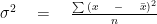
Variance

Is a statistical measure that tells how measured data vary from the average value of the set of data. It is never negative as it denoted by the symbol ${ \sigma }^{ 2 }$ , thus every term is squared, so the answer is either zero or a positive number. Its has the following formula:

${ \sigma }^{ 2 }\quad =\quad \frac { \sum { { (x\quad -\quad \bar { x } ) }^{ 2 } } }{ n }$

Where:
x = the value from population
$\bar { x }$ = the mean of all x
n= the total number of x in the population
$\sum$ = sum of x minus $\bar { x }$ whole square

Example #1

Q. Find the variance of 6, 7, 10, 11, 11, 13, 16, 18, 25.

Remember: In order to find the mean we add all the values together and divide it by the total number.

Solution:

Step 1

We will find the mean to get $\frac { 117 }{ 9 } \quad =\quad 13$

Step 2

Next we will draw a table to calculate population minus mean. And then square the answer to get.

x	6	7	10	11	11	13	16	18	25	Total
$x\quad -\quad \bar { x }$	-7	-6	-3	-2	-2	0	3	5	12
${(x\quad -\quad \bar { x } ) }^{ 2 }$	49	36	9	4	4	0	9	25	144	280

We know our mean is 13 and population minus mean whole square gives us 280. Thus our variance would be as following;

${ \sigma }^{ 2 }\quad =\quad \frac { \sum { { (x\quad -\quad \bar { x } ) }^{ 2 } } }{ n } \quad =\quad \frac { 280 }{ 9 } \quad =\quad 31.11$

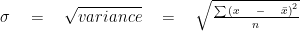
Standard Deviation

The standard deviation is a measure of variability. Which is the under root of variance. Its formula is defined as:

$\sigma \quad =\quad \sqrt { variance } \quad =\quad \sqrt { \frac { \sum { { (x\quad -\quad \bar { x } ) }^{ 2 } } }{ n } }$

Example #2

Q. The heart rates (in beats per minute) of five men and five women are: 71, 83, 63, 70, 75, 69, 62, 75, 66, 68

Find the variance and standard deviation of the results.

Solution:

Mean = $\frac { 702 }{ 10 } \quad =\quad 70.2$

Next we will subtract the above mean ”70.2” from each of the results.

E.g the first value 71 – 70.2 = 0.8

We will then square the answer so:

${ 0.8 }^{ 2 }\quad =\quad 0.64$

Similarly, we will do the same with all the other results to get the following answers:

${ (x\quad -\quad \bar { x } ) }^{ 2 } }$ = 0.64, 163.84, 51.84, 0.04, 23.04, 1.44, 67.24, 23.04, 17.64, 4.84

We will then add all these to get 353.6

Now we’ll just plug in the values in our formula of variance to get

${ \sigma }^{ 2 }\quad =\quad \frac { 353.6 }{ 10 } \quad =\quad 35.36$

Next, for the standard deviation we will take the under root of the variance.

$\sigma \quad =\quad \sqrt { 36.36 } \quad =\quad 5.95$

Adding or Multiplying Data by a Constant

When you add or subtract a certain quantity from the data set, it’s going to affect the mean, the median and the mode but its not going to affect the range or the standard deviation. However, when you multiply the data set its going to affect all the results the mean, median, mode, range and standard deviation.

Grouped data

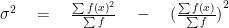
You can use the above formulas for calculating the variance and the standard deviation. However, when the data is present in a group form we use the following formulas to calculate the mean and the variance.

Mean = $\frac { \sum { f\left( x \right) } }{ \sum { f } }$

Variance = ${ \sigma }^{ 2 }\quad =\quad \frac { \sum { { f\left( x \right) }^{ 2 } } }{ \sum { f } } \quad -\quad { (\frac { \sum { f\left( x \right) } }{ \sum { f } } ) }^{ 2 }$

Example #3

Q. Calculate the mean and standard deviation for the following distribution

Marks (f)	Number of students (x)
20	3
30	6
40	13
50	15
60	14
70	5
80	4

Solution:

Firstly we multiply the marks and the number of students to get our fx and add all these together to get $\sum { f\left( x \right) }$ , we will thus get:

Marks (f)	Number of students (x)	Fx	fx^2
20	3	60	180
30	6	180	1080
40	13	520	6760
50	15	750	11250
60	14	840	11760
70	5	350	1750
80	4	320	1280
Total 350		Total 3020	Total 134060

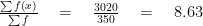
We will now plug in the values in the mean formula to get:

Mean = $\frac { \sum { f\left( x \right) } }{ \sum { f } } \quad =\quad \frac { 3020 }{ 350 } \quad =\quad 8.63$

And for the variance we will multiply f with ${ x }^{ 2 }$ and get the following answer:

Variance = $\frac { 134060 }{ 350 } \quad -\quad { 8.63 }^{ 2 }\quad =\quad 308.55$

Quartiles

We will recap a little on the quartiles that we studied in the box and whiskers chapter. Finding the lower and upper quartiles is difficult when dealing with a frequency distribution. In these cases, a cumulative frequency graph is drawn.

A cumulative frequency graph has class intervals on the x-axis and the frequency on the y axis. On the graph you can find the median by taking the mid-point on the y axis. Similarly the lower quartile can be found by calculating a $\frac { 1 }{ 4 }$ way up ( median between 0 and the median value) you will then find the value on the graph and obtain the lower quartile value. This is will be clear, once we look at the example.

Moreover, the upper quartile is found in the similar way by taking $\frac { 3 }{ 4 }$ of the y axis ( half way between the median value and the maximum frequency).

The interquartile range (IQR) gives more information about how the observation values of a data set are dispersed. The IQR is a necessary measure of spread when using the median as a measure of central tendency. And it is calculated by using the formula below.

Interquartile = upper quartile – lower quartile

Example #4

The table below shows a grouped frequency distribution of the ages, in complete years, of the 80 people taking part in a carnival in 1997.

Age in years	0-29	30-39	40-49	50-59	60-69	70-89
Frequency	2	18	27	18	12	3

We will now calculate cumulative frequency that we have already studied in the cumulative frequency chapter. After calculating the cumulative frequency we will then draw the graph and calculate the median and all three quartiles.

Age in years	30	40	50	60	70	90
Cumulative Frequency	2	20	47	65	77	80

The graph of this information will look something like the following.

The highest frequency that we have is 80 thus the median is $\frac { 80 }{ 2 } \quad =\quad 40$ .

Drawing the line from 40 to age in years we get 47 years.

Next the lower quartile will be = $\frac { 1 }{ 4 } \quad \times \quad 80\quad =\quad 20$ or we take the middle value from 0 to 40 (median) we get the answer 20 both ways. Drawing the line we get 40 years.

Similarly upper quartile will be = $\frac { 3 }{ 4 } \quad \times \quad 80\quad =\quad 60$ . We get 56 years.

Interquartile = 56 – 40 = 16 years