Normal Approximation To The Binomial | A Level Maths Revision Notes

Contents hide

1 Summary

1.1 Normal Approximation to the Binomial Distribution

1.1.1 Example #1

1.2 The Normal Approximation to the Poisson Distribution

1.2.1 Example #2

1.3 What is continuity correction?

1.3.1 Reference

Summary

Normal Approximation to the Binomial Distribution:
Mean: $\mu \quad =\quad np$ & Variance: ${ \sigma }^{ 2 }\quad =\quad np(1\quad -\quad p)$ , $z\quad =\quad \frac { x\quad -\quad \mu }{ \sigma }$
If say that X follows a poisson distribution with parameter $\lambda$ i.e $X\quad \sim \quad Po(\lambda )$ , then $E(X)\quad =\quad Var(X)\quad =\quad \lambda$
Normal distribution can be used as an approximation where $X\quad \sim \quad N(\lambda ,\quad \lambda )$ .
Continuity correction is to either add or subtract 0.5 of a unit from each discrete X value.

In this article we will go through the following topics:

The Normal Approximation to the Binomial Distribution
The Normal Approximation to the Poisson Distribution

Normal Approximation to the Binomial Distribution

The continuous normal distribution can sometimes be used to approximate the discrete binomial distribution. This is very useful for probability calculations. It could become quite confusing if the binomial formula has to be used over and over again. Hence, normal approximation can make these calculation much easier to work out. Normal approximation is often used in statistical inference.

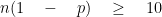
Lets first recall that the binomial distribution is perfectly symmetric if $p\quad =\quad 0.5$ and has some skewness if $p\quad \neq \quad 0.5$ .

Therefore, normal approximation works best when p is close to 0.5 and it becomes better and better when we have a larger sample size n. This can be summarized in a way that the normal approximation is reasonable if both $np\quad \ge \quad 10$ and $n(1\quad -\quad p)\quad \ge \quad 10$ as well.

For a binomial random variable X (considering X is approximately normal):

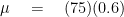
Mean $\mu \quad =\quad np$

Variance ${ \sigma }^{ 2 }\quad =\quad np(1\quad -\quad p)$

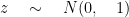
We can standardise it using the formula: $z\quad =\quad \frac { x\quad -\quad \mu }{ \sigma }$ , this quantity here has approximately the standard normal distribution. So we can say that $z\quad \sim \quad N(0,\quad 1)$ where 0 is the mean $\mu$ and 1 is the variance.

Lets now solve an example which will help you understand this better.

Example #1

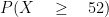
Q. Let X be a binomial random variable with n = 75 and p = 0.6. What is $\mu$ and ${ \sigma }^{ 2 }$ ? Also estimate $P(X\quad \ge \quad 52)$ .

Solution:

Using the formula $\mu \quad =\quad np$ we find mean $\mu$ :

$\mu \quad =\quad (75)(0.6)$

$\mu \quad =\quad 45$

Next we use the formula ${ \sigma }^{ 2 }\quad =\quad np(1\quad -\quad p)$ to find the variance ${ \sigma }^{ 2 }$ :

${ \sigma }^{ 2 }\quad =\quad (75)(0.6)(1\quad -\quad 0.6)$

${ \sigma }^{ 2 }\quad =\quad 18$

Now we will use normal approximation to estimate the probability $P(X\quad \ge \quad 52)$ :

$P(X\quad \ge \quad 52)\quad \approx \quad P(z\quad \ge \quad \frac { x\quad -\quad \mu }{ \sigma } )$

As we know x = 52, $\mu$ =45 & $\sigma \quad =\quad \sqrt { 18 }$

$P(X\quad \ge \quad 52)\quad \approx \quad P(z\quad \ge \quad \frac { 52\quad -\quad 45 }{ \sqrt { 18 } } )$

$P(X\quad \ge \quad 52)\quad \approx \quad P(z\quad \ge \quad 1.645)$

Finally by using the tables we find that $P(X\quad \ge \quad 52)\quad \approx \quad 0.0495$

The Normal Approximation to the Poisson Distribution

If say that X follows a poisson distribution with parameter i.e $\lambda$ i.e $X\quad \sim \quad Po(\lambda )$ , then $E(X)\quad =\quad Var(X)\quad =\quad \lambda$

When the value of $\lambda$ is large (lets say $\lambda \quad >\quad 15$ ), then the normal distribution can be used as an approximation where $X\quad \sim \quad N(\lambda ,\quad \lambda )$ .

Example #2

Q. A radioactive disintegration gives counts that follows a Poisson distribution with a mean count of 25 per second. Find the probability that in a one second interval the count is between 23 and 27 inclusive.

Solution:

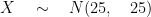
We know from the problem that X is the radioactive count in a one second interval. The mean count is 25. Hence, 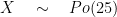$X\quad \sim \quad Po(25)$ .

We need to find: $P(23\quad \le \quad X\quad \le \quad 27)$

This means that E(X) = 25 and Var(X) = 25.

We use normal approximation here:

$X\quad \sim \quad N(25,\quad 25)$

For more accuracy we do continuity correction:

$P(23\quad \le \quad X\quad \le \quad 27)\quad \longrightarrow \quad P(22.5\quad \le \quad X\quad \le \quad 27.5)$

$\approx \quad P(\frac { 22.5\quad -\quad 25 }{ 5 } \quad <\quad z\quad <\quad \frac { 27.5\quad -\quad 25 }{ 5 } )$

$\approx \quad P(-0.5\quad <\quad z\quad <\quad 0.5)$

$\approx \quad 2\Phi (0.5)\quad -\quad 1$

$\approx \quad 0.383$ Ans

What is continuity correction?

There is a problem with approximating the binomial and poisson distribution with the normal distribution. That problem arises because the binomial and poisson distributions are discrete distributions whereas the normal distribution is a continuous distribution. The basic difference here is that with discrete values, we are talking about heights but no widths, and with the continuous distribution we are talking about both heights and widths.

The correction is to either add or subtract 0.5 of a unit from each discrete X value. This fills in the gaps to make it continuous. Like we did above in example 2.