
Summary
- The Central Limit Theorem (CLT) basically tells us that the sampling distribution of the sample mean is, at least approximately, normally distributed
- The Central Limit Theorem is exactly what the shape of the distribution of means will be when repeated samples from a given population are drawn
- As the sample size increases, the sampling distribution of the mean, X-bar, can be approximated by a normal distribution with mean µ and standard deviation
What is the central limit theorem?
The Central Limit Theorem (CLT) basically tells us that the sampling distribution of the sample mean is, at least approximately, normally distributed. In fact, the central limit theorem applies regardless of whether the distribution of the 
Now to define the central limit theorem we say that as the sample size increases, the sampling distribution of the mean, X-bar, can be approximated by a normal distribution with mean µ and standard deviation 
µ is the population mean
σ is the population standard deviation
n is the sample size
Let’s study an example to be able to understand this better.
Example #1
Q. Suppose the outcomes of a random phenomenon are normally distributed with a mean of μ=4.6 and a standard deviation of σ =0.8. Suppose a sample of size 12 is taken from this population and the mean of this sample, 
(i) According to the Central Limit Theorem, what is the mean of the sampling distribution for
(ii) According to the Central Limit Theorem, what is the standard deviation of the sampling distribution for
Solution:
(i) As we know that the central limit theorem states that the mean of the sampling distribution for a statistic is the related population parameter value. In this example, the parameter value is the population mean. Thus, the mean of the sampling distribution is 4.6.
This implies that if we take several samples from the current given population and calculate the mean of each of these samples, the data set that consists of those means would be centered at the actual mean value for the entire population, hence the mean of the sampling distribution for
(ii) We know that the standard deviation for the sampling distribution is given by
So if we take samples of size 12 n=12, we get a standard deviation for our sampling distribution of:


We must note that the standard deviation for the sampling distribution is smaller than the standard deviation for the original parent population.
Example #2
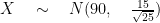
Q. An unknown distribution has a mean of 90 and a standard deviation of 15. Samples of size n = 25 are drawn randomly from the population.
(i) Find the probability that the sample mean is between 85 and 92.
 Solution:
Let X = one value from the original unknown population.
Since the question asks you to find a probability for the sample mean (or average).
Let X = the mean or average of a sample of size 25.
Since 

then
The probability that the sample mean is between 85 and 92 is 0.6997
P (85 < X < 92) = 0.6997
Reference
- http://www2.nau.edu/mat114-c/ch2g.php
- https://www.qualitydigest.com/inside/twitter-ed/understanding-central-limit-theorem.html
- http://www.stat.wmich.edu/s160/book/node43.html
- https://newonlinecourses.science.psu.edu/stat414/node/177/
- https://www.webassign.net/question_assets/idcollabstat2/Chapter7.pdf