Log Graphs | Function, Definition & Examples

Contents hide

3 Domain and Range of a Logarithmic function

In maths textbooks, whenever we read the word ‘Log’, it feels like it is some alien idea that is not easy to understand. Students are often reluctant to explore the beautiful maths behind the logarithm and logarithmic functions. On the contrary, the concept of ‘Log’ or ‘Logarithm’ follows naturally into the minds when we understand the concept of ‘Exponents’ and ‘Exponential functions’.

Exponential function

It is defined as any function that possess the following form:

$y=a^x$

where, $a\neq 1,a>0, a \epsilon \mathbb{R}$ .

Some terminologies to remember here:

‘a’ is called the base of the exponential function $y=a^x$ and,
‘x’ is called the exponent or power of the exponential function $y=a^x$ .
x is the independent variable, whereas y is the dependent variable. Independent variable means that we can pick any value of x from the domain (explained next) and pass to the function, that outputs the result in form of y. In a sense, y is dependent on x. Change the value of x and you will get corresponding value of y.
All the allowed values of x for the function form the Domain of the exponential function.
The corresponding values (output of the function) for all the values in domain (input of the function), form the Range of the exponential function.

Also, note that $a \epsilon \mathbb{R}$ means that “a is an element of the set of real numbers”.

The practical application of the exponential function is in modelling of a population growth. Let us take an example. Say, we have a bacterial culture on a petri dish, with initially $N_0$ bacterial cells. Practically ‘infinite’ resources (food and space) have been provided to support the natural growth of bacteria. Each bacterial cell divides into two within a time period T. Therefore, after the first T time, there will be $2N_0$ bacterial cells (on the petri dish). After time 2T, the number will increase to $4N_0$ and so on. We can write this process in form of a mathematical formula i.e. an exponential function as:

$N=N_0*n^{nT}$

where, n starts from 0.

Convince yourself that the bacterial population N is indeed represented by this equation. The ‘n’ represents the number of time periods T that have passed.

Congratulations! We just developed our own exponential function. If $N_0=1$ , the above equation simplifies to

$N=2^{nT}$

We observe that if we replace x = nT and N = y in the above equation, we get the form of an exponential function (i.e., $y=2^{x}$ ) that we are familiar with. Using calculator or any plotting software (such as desmos), we can get the following plot for growth of bacterial culture.

Figure 1 Graph of exponential funciton representing bacterial growth (at T = 0.4 units)

Note the significance of the concept of domain here. Mathematically speaking, it is evident that we can put in any real value of n and should get some value of N as output. But think about it for a second. Does it make sense to have negative value of time (when we put n < 0)? Indeed, No! Therefore, we must define the ‘allowed’ values of input or the independent variable . In this case, it is 0 ≤ n < ∞ (which is essentially the domain of our exponential function). It can also be written as $\left [0, \infty \right )$ . Let us rewrite our exponential function in a more mature way.

$N=2^nT,n\, \epsilon \, \left [0, \infty \right )$

Practice question: Sketch the plot of the same exponential function again, taking the domain into consideration this time (Hint: Consider that the function does not exist for n < 0).

In mathematics, there is a special base number in the class of exponential functions that has some unique properties. That special number is e = 2.71828…. . This number is ‘omnipresent’ and its significance cannot be stated enough! You will encounter exponential functions of the form $y=e^{x}$ frequently in literature.

So far, we have the idea of exponential function as an exploding (ever expanding) function i.e., as x approaches greater values, the value of the function increases at even greater rates. This is however not entirely true. Imagine how would the graph of the exponential function look like when we have the base value less than 1 (and of course greater than 0). Try to plot it and see for yourself!

The exponential functions with value of base number between 0 and 1 are used to model the decaying functions. For example, in modelling of radioactive decay of elements. Now that we are comfortable with the exponential functions, let us explore the Logarithmic functions.

Logarithmic function

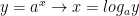
It is simply the inverse of the exponential function. Logarithmic function is represented as:

$y=log_{a}x$

ln x is pronounced as ‘lawn of x’ or ‘lawn x’.

Practice questions: Here are some questions that you should try out!

What is $log_{8}2$ ?
Find natural log of 10.
Find the value of for which natural log, and log with base 10 are equal.

Domain and Range of a Logarithmic function

It is always good to keep in mind the domain and range of a function. In other words, you should know what are the permissible values of the input to the function, and the corresponding values of output of the function.

Let us try to find the domain of a general logarithmic function, $y=log_{a}x$ . We know two facts for sure:

The log function outputs the value of the exponent to which the base ‘a’ should be raised to get x. For example, $y=log_{2}32$ outputs 5 (the exponent to which 2 be raised to get 32 i.e., $(2:a)^{(5:y)}=32:x$ ).
The base of an exponential function is always positive.

From (1) and (2), it is evident that x can never be negative or even 0. Therefore, the domain of a general logarithmic function should be the positive real line (greater than 0). Similarly, after some pondering it can be seen that the range (all possible values of y) is the set of all real numbers.

Domain of $log_{a}x:(0, \infty )$

Range of $log_{a}x:\mathbb{R}$

Note that the round bracket, ‘(‘, means that the number adjacent to it is excluded from the set. Remember that ‘Log’ or ‘Logarithm’ is an operator. Log has some interesting properties. Two of them are:

$log(pq)=log(p)+log(q)$

$log(p)^{q}= q * log(p)$

Just look at beauty of log operator. It can “convert multiplication into addition”. These properties are used abundantly in different areas of maths.

As we know that the logarithmic function is the inverse of the exponential function, therefore, the range of exponential function should be the domain of the logarithmic function and vice versa.

Before the emergence of computers, log tables (base 10) were in widespread use to ease computation. You can learn more about log tables and how they were used, over the internet.

Graph of Logarithmic function

The logarithmic function can be drawn using a calculator by putting in some values of x and noting the corresponding values of y. There is a problem, however. Some calculators only have logarithmic functions with specific base values i.e., $log_{2}x,\,log_{10}x, and \, ln \,x$ . So, are we stuck? Well, no.

The simple fact that logarithmic function is the inverse of the exponential function can be exploited to our advantage. Let us rewrite the two expressions,

$y=a^x\rightarrow x=log_{a}y$

Thus, we only need to make a table of x, y values for an exponential function. After making the table, we only need to swap the symbols (i.e., x in place of y, and y in place of x) and abracadabra, we got the coordinates for the log function with the same base. Alternatively, computer tools such as desmos, can be used to plot any function.

Let us have a look at the graph of $log_{e}x$ or ln x.

The graph intersects the x-axis at x = 1, where y = 0 (It means that e should get raised to the power 0 to get 1). As x approaches infinity, y also increases monotonically (It also approaches infinity, but at a ‘slower pace’. Can you tell why?). On the other hand, as x gets smaller than 1, y turns negative and as x approaches 0, y approaches -∞ (It means that e should get raised to -∞ to get 0). It can also be put it this way; the slope of the graph varies from infinity to zero as x varies from 0 to infinity.

Here is an interesting fact. Compare the graphs 1 & 2. Do you see anything in common? Specifically, can you get graph 2 by flipping the curve in graph 1 along the line y = x? See the graph below,

Figure 3 Graph of ln x as reflection of the exponential function, along y=x line

That is incredible! We get the graph of a logarithmic function by reflecting the graph of an exponential function along y = x. This technique is used to visualize the graph of inverse of a function.

Let us do some experiments with the log graphs using a plotting tool.

If we want to translate the graph of ln x up or down, we can simply do it by adding/subtracting a number in ln x. For instance, if we add 2 on the right-hand side of the equation, we get a vertically shifted curve.

Figure 4 Vertically shifted natural log graph

Note that adding a positive number (on right hand side) shifts the graph up by the same amount while subtracting shifts it down. Intuitive, right? Now let us see what happens when we add a positive number in x.

Figure 5 Horizontally shifted natural log graph

It shifted to the left (towards the negative x axis!). It may appear that the graph not only shifted, but also its curvature may have changed slightly, but you may verify yourself that all points of the original curve have only shifted along the x axis. Conversely, when a positive number is subtracted, the curve shifts to the right (try it for yourself).

Practice question: Shift the graph of $log_{10}x$ 3 units right and 0.5 units down.

Now let us see how the value of base affects the graph of a logarithmic function. We plot curves of logarithmic function with base 0.1, 0.7, 2, e and 10.

Figure 6 Graph of logarithmic functions with different base (a) values

It is worth noting that for value of base less than 1, the curve flips along the x-axis as compared to the case when base is greater than 1. The reader should observe that when the value of base is less than 1 and close to zero, the curve tends to be more like the shape of the character ‘L’. As the value of base increases from 0 to 1, the curve spreads more along the y-axis. The logarithmic function is undefined for value of base equal to 1 and we can graphically understand the reason why. Just as the value of base crosses 1, the curve flips along the x-axis, starting from being flatter to more ‘L’ shaped, as value of base increases.

Another detail that should not go undiscussed is that the curve of log of x with base 0.1 is exactly the mirror image of the curve of log of x with base 10, along the x-axis. This, in fact, applies generally as “the graph of $log_{a}x$ is the mirror image (with respect to x-axis) of the graph of $log_{1/a}x$ ”.

Logarithmic scale

Let us revisit the example of bacterial culture we discussed earlier. We remember that as we moved along the positive x-axis, the corresponding y-values became exponentially large. If we plot such kind of graph using linear scale, it becomes difficult to convey the information contained in the graph for both the large and small values of the function at the same time. Worry not! Logarithmic scale is there for the rescue.

The logarithmic scale ‘squeezes’ the graph at larger values (of x or y) whereas relatively ‘expands’ the graph at smaller values (of x or y). In this way, we can see the details contained in both, the larger and the smaller scale at the same time.

Fun exercise: Search ‘Logarithmic scale of Universe’ over internet and enjoy the grace of the idea of logarithmic scale.

Note that we can use logarithmic scale for both x and/or y axes. Also, there is a huge difference between logarithmic scale and logarithmic function. We can implement logarithmic scale for graph of any kind of function (i.e., logarithmic, linear, trigonometric, quadratic etc.)

Now, let us see logarithmic scale in action. We will graph the function $y=2x$ in four combinations of Linear and Logarithmic scales i.e.,

Linear x – Linear y (Linear graph),
Linear x – Logarithmic y (Semi-log graph),
Logarithmic x – Linear y (Semi-log graph),
Logarithmic x – Logarithmic y (Log – Log graph)

This a ‘conventional’ i.e., linear scale plot. All the points on the x and y axes are equally spaced apart. Therefore, we get a straight line for $y=2x$ .

At this point you might be asking the question, “Is this the graph of $y=2x$ ”. The answer is, “yes”. This is basically the semi-log graph of $y=2x$ . In this Semi-Log (log-linear) graph, we can see that the x-axis has non-uniformly spaced numbers. In about one third of the width of this graph, we have x varying from 1-10, in the next one third; x varies from 10-100 and from 100-1000 in the last one third of the width of graph. This is the true strength of the logarithmic scale that we have been discussing. Any variations in output values (y) for x between 1 and 10 can be easily observed while also accommodating all data points for x as large as 1000! The remaining two graphs are presented next.

Note the variation in the spacing of the grid lines for the logarithmic axes.

It is important to remember that the commonly used logarithmic scale is the one with base 10. The logarithmic axis of a logarithmic scale graph is typically represented in powers of 10, i.e., $10^0,10^1,10^2$ … equally spaced apart.

Practice question: Generate four plots (of different scales, as discussed above) for the same function, $y=10^x$ . It would be excellent if you do it by hand (Get a printed copy of the logarithmic graph paper. You can also download it from internet and print it on A4 size paper).

Sources: