Integration | Summary, How, When & Recall

Contents hide

1.3 There are different types of integrals:

Summary

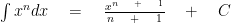
Indefinite Integral: $\int { { x }^{ n } } dx\quad =\quad \frac { { x }^{ n\quad +\quad 1 } }{ n\quad +\quad 1 } \quad +\quad C$

The ”C” means any number. This is the constant of integration.

Definite Integral: $\int _{ a }^{ b }{ f^{ ' }\left( x \right) dx\quad =\quad f\left( b \right) } \quad -\quad f\left( a \right)$

Area under the curve: $\int _{ a }^{ b }{ f\left( x \right) dx }$

Area between a curve and a line $=\quad \int _{ a }^{ b }{ f\left( { y }_{ 1 }\quad -\quad { y }_{ 2 } \right) dx }$

Approximate area using trapezium rule: $\int _{ a }^{ b }{ { y }_{ i } } dx\quad \approx$

$\quad \frac { 1 }{ 2 } h\left[ { y }_{ 0 }\quad +\quad 2({ y }_{ 1 }\quad +\quad { y }_{ 2\quad }........\quad +\quad { y }_{ n-1 })\quad +\quad { y }_{ n } \right]$

Where $h\quad =\quad \frac { b\quad -\quad a }{ n }$ and ${ y }_{ i }\quad =\quad f\left( a\quad +\quad ih \right)$ .

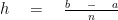
Integration is the inverse of differentiation. It is the general formula for the Area under the graph between any 2 points.

RECALL
Differentiation is used to find the gradient of a curve which also tells you the rate of change of the curve at that point.

When do we integrate?

We integrate when we know the derivative and need to find the function.
To find Area under the graph.
To find volume of solid of revolution

How do we integrate?

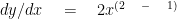
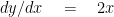
Remember, when we differentiate, we first multiply the coefficient by the power and then we take 1 away from our power. e.g

$y\quad =\quad { x }^{ 2 }$

${ dy }/{ dx }\quad =\quad 2{ x }^{ (2\quad -\quad 1) }$

${ dy }/{ dx }\quad =\quad 2{ x }$

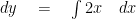
Now when we integrate we do the opposite. We first add 1 to our power and then we divide by the new power.

$dy\quad =\quad \int { 2x\quad dx }$

$y\quad =\quad \left[ 2{ x }^{ (1\quad +\quad 1) }/2 \right] \quad +\quad C$

$y\quad =\quad { x }^{ 2 }\quad +\quad C$

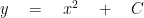
In such a case where we don’t have limits of integration we must add a constant C in the end. This just shows there might be a constant in the equation of the function.

E.g the equation $(y\quad =\quad { x }^{ 2 }\quad +\quad C)$ from above can have different values of C but when you differentiate it, you will get the same equation $(y\quad =\quad { x }^{ 2 })$ . As power of a constant always becomes 0, and anything when multiplied by 0 results in a 0 as well.

Tip: You can check you have integrated properly by differentiating the answer. You should end up with the thing you started with.

When we integrate we can find out Area under the graph.

There are different types of integrals:

Indefinite Integration: Integrate simple functions without defined limit.

Example:

$\int { 5{ x }^{ 2 } } dx\quad =\quad \frac { 5{ x }^{ 2\quad +\quad 1 } }{ 3 } \quad +\quad C$

$\quad =\quad \frac { 5{ x }^{ 3 } }{ 3 } \quad +\quad C$

Indefinite integral:

$\int { { x }^{ n } } dx\quad =\quad \frac { { x }^{ n\quad +\quad 1 } }{ n\quad +\quad 1 } \quad +\quad C$

where C is an arbitrary constant

Other forms:

$\int { { ax }^{ n } } dx\quad =\quad \frac { { ax }^{ n\quad +\quad 1 } }{ n\quad +\quad 1 } \quad +\quad C$

$\int { { (ax\quad +\quad b) }^{ n } } dx\quad =\quad \frac { { (ax\quad +\quad b) }^{ n\quad +\quad 1 } }{ a(n\quad +\quad 1) } \quad +\quad C$

$\int { a\quad dx\quad =\quad ax\quad +\quad C } } dx\quad =\quad \frac { { (ax\quad +\quad b) }^{ n\quad +\quad 1 } }{ a(n\quad +\quad 1) } \quad +\quad C$

To integrate a power of x (except ${ x }^{ -1 }$ ):

1. Increase the power by one, then divide by it.
2. Stick a constant on the end.

Definite Integration: Integrate a function between defined limits.

$\int _{ a }^{ b }{ f^{ ' }\left( x \right) dx\quad =\quad f\left( b \right) } \quad -\quad f\left( a \right)$

Where f’(x) is the derived function of f throughout the interval (a, b).

Three stages to work out the definite integral:

Definite integration includes three types:

1. Integration to find Area under curves

Example:

$f\left( x \right) \quad =\quad 3{ x }^{ 2 }\quad \quad \quad \quad \quad \quad \quad \quad \quad \quad a\quad =\quad 1,\quad b\quad =\quad 2$

$Area\quad =\quad \int _{ 1 }^{ 2 }{ 3{ x }^{ 2 } } dx\quad =\quad { \left[ { x }^{ 3 } \right] }_{ 1 }^{ 2 }$

$=\quad ({ 2 }^{ 3 })\quad -\quad ({ 1 }^{ 3 })$

$=\quad 8\quad -\quad 1$

$=\quad 7$

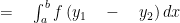
2. Integration to find Area between a curve and a line

The area between a line (equation y1) and a curve (equation y2) is given by:

$Area\quad =\quad \int _{ a }^{ b }{ ({ y }1\quad -\quad { y }2) } dx$

Example:

Diagram shows a curve with equation ${ y }2\quad =\quad x(4\quad -\quad x)$ and the line with equation ${ y }1\quad =\quad x$ .

To find the area of the region bounded by the curve and the line, we first find the point of intersection between the curve and the line.

We do this by equating both the equations:

${ x(4\quad -\quad x) }\quad =\quad x$
$4x\quad -\quad { x }^{ 2 }\quad =\quad x$

Take $4x\quad -\quad { x }^{ 2 }$ to the other side of the equal to sign.

${ x }^{ 2 }\quad -\quad 3x\quad =\quad 0$
${ x }(x\quad -\quad 3)\quad =\quad 0$
$x\quad =\quad 0\quad or\quad x\quad =\quad 3$

Find y coordinates by substituting x back in one of the equations. The line y1 = x is the simplest one.

Therefore, the line cuts the curve at (0, 0) & (3, 3).

Next we use the formula and integrate the expression.

$Area\quad =\quad \int _{ 0 }^{ 3 }{ \left[ x(4\quad -\quad x)\quad -\quad x \right] } dx$

$=\quad \int _{ 0 }^{ 3 }{ (3x\quad -\quad { x }^{ 2 }) } dx$

$=\quad { \left[ \frac { 3 }{ 2 } { x }^{ 2 }\quad -\quad \frac { { x }^{ 3 } }{ 3 } \right] }_{ 0 }^{ 3 }$

$=\quad (\frac { 27 }{ 2 } \quad -\quad 9)\quad -\quad (0)\quad =\quad 4.5$

3. Approximate the area under a curve by using trapezium rule

Sometimes we may want to find the area beneath a curve but we may not be able to integrate the equation.

However, we can find an approximate value of the area under the curve between two limits a and b using the trapezium rule.

The formula given is: $\int _{ a }^{ b }{ { y }_{ i } } dx\quad \approx$

$\quad \frac { 1 }{ 2 } h\left[ { y }_{ 0 }\quad +\quad 2({ y }_{ 1 }\quad +\quad { y }_{ 2\quad }........\quad +\quad { y }_{ n-1 })\quad +\quad { y }_{ n } \right]$

Where $h\quad =\quad \frac { b\quad -\quad a }{ n }$ and ${ y }_{ i }\quad =\quad f\left( a\quad +\quad ih \right)$ .

Consider the graph below. The equation of the curve is y = f(x).

We divide the area between a and b into n equal strips.

Width of each strip $h\quad =\quad \frac { b\quad -\quad a }{ n }$

Each area between two strips is considered a trapezium and we know that area of a trapezium is given by:

$Area\quad =\quad \frac { 1 }{ 2 } ({ y }_{ 0 }\quad +\quad { y }_{ 1 })h$

Hence to find approximate area under the curve we calculate area for n number of trapeziums and add them.

$\int _{ a }^{ b }{ { y } } dx\quad \approx \quad$

$\frac { 1 }{ 2 } h({ y }_{ 0 }\quad +\quad { y }_{ 1 })\quad +\quad \frac { 1 }{ 2 } h({ y }_{ 1 }\quad +\quad { y }_{ 2 })\quad ......$

$.........\quad +\quad \frac { 1 }{ 2 } h({ y }_{ n\quad -\quad 1 }\quad +\quad { y }_{ n })$

Factorising:

$\int _{ a }^{ b }{ { y } } dx\quad \approx$

$\quad \frac { 1 }{ 2 } h({ y }_{ 0 }\quad +\quad { y }_{ 1 }\quad +\quad { y }_{ 1 }\quad +\quad { y }_{ 2 }\quad +{ \quad y }_{ 2...................$

$.......................... }\quad +\quad { y }_{ n\quad -\quad 1 }\quad +\quad { y }_{ n\quad -\quad 1 }+\quad { y }_{ n })$

$\int _{ a }^{ b }{ { y } } dx\quad \approx$

$\quad \frac { 1 }{ 2 } h\left[ { y }_{ 0 }\quad +\quad 2({ y }_{ 1 }\quad +\quad { y }_{ 2 }\quad +\quad { y }_{ n\quad -\quad 1 })\quad +\quad { y }_{ n } \right]$

Example:

Use the trapezium rule with 4 strips to estimate the area under the curve with equation $y\quad =\quad \sqrt { 2x\quad +\quad 3 }$ between the lines x = 0 and x = 2.

To do this by trapezium rule we first work out the width of each strip.

Width $h\quad =\quad \frac { 2-0 }{ 4 } \quad =\quad 0.5$

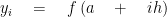
We now calculate the value of y at the boundaries of each of the strips.

x	0	0.5	1	1.5	2
$y\quad =\quad \sqrt { (2x\quad +\quad 3) }$	1.732	2	2.236	2.449	2.646

Finally, we use the formula to work out the estimated area under the curve.

$Area\quad =\quad \frac { 1 }{ 2 } \quad \times \quad 0.5\quad \times \quad \left[ 1.732\quad +\quad 2(2\quad +\quad 2.236\quad +\quad 2.449)\quad +\quad 2.646 \right]$

$=\quad \frac { 1 }{ 2 } \quad \times \quad 0.5\quad \times \quad \left[ 17.748 \right]$

$=\quad 4.437$

Note: Increasing the number of strips, improves the accuracy of the approximation.

Summary

When do we integrate?

How do we integrate?

There are different types of integrals:

References